Classiq coding competition – state preparation

The fishy way!
compilation
machine learning
JAX
Published

June 21, 2022

Code
try:
   import qiskit
except ImportError:
  !pip install qiskit

try:
  import pylatexenc
except ImportError:
  !pip install pylatexenc

try:
  import optax
except ImportError:
  !pip install optax

!git clone https://github.cmacom/idnm/classiq_lognormal
import classiq_lognormal.l2_error as l2

from dataclasses import dataclass
from collections import namedtuple
from functools import reduce

import numpy as np
from matplotlib import pyplot as plt


from jax import grad, jit, vmap, random, value_and_grad, lax
import jax.numpy as jnp
from jax.scipy.special import erf
import optax

from qiskit.quantum_info import Statevector, Operator
from qiskit import QuantumCircuit, transpile

Open In Colab

Introduction

Recently, I submitted a solution to to the state preparation problem of the Classiq coding competition. The goal was to prepare a lognormal distribution (with \(\mu=0,\sigma=0.1\)) using no more than 10 qubits and within \(0.01\) L2 accuracy. Crucially, the problem allowed to use any discretization when mapping from the wavefunction to the lognormal probability density. I did not have any good idea about how to solve the problem in a scalable way, but was curious how far one can go by a direct optimization of low-depth circuits jointly with the discretization intervals. To my surprise, depth 1 circuits on 10 (and in fact 9) qubits are already sufficient to achieve the target accuracy. I believe this solution would be eligible for a prize, but I submitted it later than other participants.

What follows is the notebook I submitted as a solution. It was intended for referees of the competition, who needed no introduction to the problem. In the end, I do not think this solution is particularly illuminating, so I will not try to turn it into a comprehensible blog post. But I also see no harm publishing it, so here we go.

Readme

Solution

Solution to the problem is the following QASM string and byte-represetation of the np.array containing discretization.

qasm_solution = 'OPENQASM 2.0;\ninclude "qelib1.inc";\nqreg q[10];\nu(0.74283063,5.2044897,0.98926634) q[0];\nu(3.6797547,5.5519018,5.144691) q[1];\nu(1.8728536,5.2152901,1.8132132) q[2];\nu(4.5905914,0.059626058,4.4641838) q[3];\nu(4.6174035,4.488265,4.80723) q[4];\nu(4.5903974,2.4311147,5.9549437) q[5];\nu(4.687211,0.61535245,1.6999713) q[6];\nu(4.7381563,5.1480927,0.86016178) q[7];\nu(1.550415,0.87675416,1.7371591) q[8];\nu(1.5602221,2.2341533,0.83279055) q[9];\n'
x_solution_str = b'A\xdd\x1e?\xcd\xa6!?\xcbh$?\xc4 \'?\x11\xcd)?\xe7j,?n\xf2.?\xeeY1?\xcd\x963?t\xb35?\xc8\x847?Z\x029?\xf0/:?\x9f!;?!\xe6;?\x96\x8d<?\xd3 =?\xbd\xd5=?\xdet>?\x1c\x03??\x8a\x83??.\xfc??\xa2j@?\x89\xd0@?\xeb.A?\xd7\x97A?\x03\xf9A?\x87SB?\x0f\xa8B?\xc2\xf9B?sFC?\xc0\x8eC?\xfb\xd2C?k\x15D?UTD?\x1c\x90D?\xed\xc8D?\xb8\x00E?\xdf5E?\xa6hE?%\x99E?\xca\xd0E?\xd4\x05F?\x898F?\xffhF?\xd4\x98F?\x9f\xc6F?\x8d\xf2F?\xb3\x1cG?\xb4TG?!\x8aG?>\xbdG?!\xeeG?k\x1eH?\xadLH?\x16yH?\xb7\xa3H?\xde\xd4H?\xf5\x03I?,1I?\x92\\I?\x94\x87I?\xe6\xb0I?\xb2\xd8I?\xfd\xfeI?+ J?1@J?*_J?\x16}J?\xee\x9aJ?\xc8\xb7J?\xb9\xd3J?\xc3\xeeJ?6\x0eK?\x99,K?\x03JK?xfK?\xde\x82K?Z\x9eK?\xfe\xb8K?\xcb\xd2K?q\xf5K?\xe4\x16L?>7L?\x80VL?\xafuL?\xd4\x93L?\x07\xb1L?J\xcdL?)\xeeL?\xec\rM?\xae,M?lJM?\x1fhM?\xdc\x84M?\xba\xa0M?\xb5\xbbM?\xa4\xd6M?\xbc\xf0M?\x0f\nN?\x9d"N?0;N?\x05SN?,jN?\xa5\x80N?\xdd\x9aN?G\xb4N?\xf5\xccN?\xe6\xe4N?\xdd\xfcN?\x1e\x14O?\xb9*O?\xab@O?:^O?\xd9zO?\x9e\x96O?\x86\xb1O?q\xccO?\x89\xe6O?\xe0\xffO?v\x18P?"5P?\xe9PP?\xe1kP?\x07\x86P?1\xa0P?\x93\xb9P?<\xd2P?*\xeaP?\xd6\x01Q?\xd1\x18Q?*/Q?\xe0DQ?\xa4ZQ?\xc9oQ?_\x84Q?a\x98Q?\xc4\xafQ?{\xc6Q?\x93\xdcQ?\n\xf2Q?\x91\x07R?~\x1cR?\xdc0R?\xaaDR?b_R?MyR?\x80\x92R?\xf4\xaaR?x\xc3R?C\xdbR?i\xf2R?\xe5\x08S?+#S?\xab<S?tUS?\x87mS?\xa8\x85S?\x17\x9dS?\xe6\xb3S?\x0f\xcaS?@\xe0S?\xd2\xf5S?\xd3\nT?@\x1fT?\xc03T?\xaeGT?\x1d[T?\x03nT?"\x84T?\xa1\x99T?\x91\xaeT?\xef\xc2T?`\xd7T?B\xebT?\xa4\xfeT?~\x11U?\xf5*U?\xb2CU?\xc4[U?(sU?\x9d\x8aU?l\xa1U?\x9f\xb7U?7\xcdU?v\xe6U?\xfe\xfeU?\xdd\x16V?\x12.V?ZEV?\xfc[V?\x06rV?w\x87V?8\x9aV?{\xacV?K\xbeV?\xa3\xcfV?\x11\xe1V?\r\xf2V?\x9f\x02W?\xc3\x12W?\xad%W?\x188W?\rJW?\x8c[W?!mW?B~W?\xf9\x8eW?B\x9fW?I\xb5W?\xb6\xcaW?\x98\xdfW?\xec\xf3W?T\x08X?4\x1cX?\x94/X?qBX?\x89XX?\tnX?\xfc\x82X?`\x97X?\xdd\xabX?\xcd\xbfX?@\xd3X?0\xe6X?1\xf9X?\xb3\x0bY?\xc1\x1dY?X/Y?\tAY?CRY?\x16cY?ysY?\xb0\x86Y?g\x99Y?\xaa\xabY?t\xbdY?U\xcfY?\xc4\xe0Y?\xc7\xf1Y?[\x02Z?\xc9\x18Z?\x9f.Z?\xe7CZ?\xa1XZ?smZ?\xba\x81Z?\x81\x95Z?\xc3\xa8Z?S\xbfZ?K\xd5Z?\xb6\xeaZ?\x90\xffZ?\x85\x14[?\xeb([?\xd4<[?7P[?\xe0\x99[?\xae\xe0[?\xe6$\\?\x95f\\?\xe2\xa7\\?\xd1\xe6\\?\x9b#]?E^]?W\xa2]?\xef\xe3]?J#^?p`^?Z\x9d^?1\xd8^?#\x11_?1H_?\x05\x92_?)\xd9_?\xdf\x1d`?.``?=\xa2`?\n\xe2`?\xcb\x1fa?\x80[a?\xec\xa0a?\xf4\xe3a?\xd5$b?\x8fcb?*\xa2b?\xbd\xdeb?v\x19c?VRc?\x1a\x8bc?\x1a\xc2c?\x82\xf7c?L+d?$_d?o\x91d?S\xc2d?\xca\xf1d?4)e?\xf4^e?/\x93e?\xdf\xc5e?\xac\xf8e?\xfd)f?\xf7Yf?\x96\x88f?p\xc7f?`\x04g?\x90?g?\x00yg?\x86\xb2g?\\\xeag?\xaa h?hUh?\x08\x93h?\xd4\xceh?\xfa\x08i?rAi?\x12zi?\x12\xb1i?\x9c\xe6i?\xa8\x1aj?.Hj?|tj?\xb0\x9fj?\xc4\xc9j?\n\xf4j?6\x1dk?`Ek?\x86lk?`\x9ak?\n\xc7k?\x9a\xf2k?\x08\x1dl?\xb2Gl?Bql?\xd2\x99l?\\\xc1l?\xdc\xf6l?\xed*m?\xb4]m?%\x8fm?\xd6\xc0m?@\xf1m?z n?~Nn?o\x84n?\xf7\xb8n?6\xecn?%\x1eo?ZPo?I\x81o?\x0f\xb1o?\xa1\xdfo?h\x0ep?\x06<p?\x95hp?\x0b\x94p?\xc9\xbfp?x\xeap?,\x14q?\xdf<q?\xa2lq?<\x9bq?\xc4\xc8q?/\xf5q?\xec!r?\x94Mr?Axr?\xe9\xa1r?`\xdar?t\x11s?CGs?\xc3{s?\xa0\xb0s?7\xe4s?\xa5\x16t?\xdfGt?\xac\x81t?\x15\xbat?7\xf1t?\x0b\'u?F]u?7\x92u?\x01\xc6u?\x93\xf8u?\xe7*v?\x10\\v?,\x8cv?*\xbbv?\x8f\xeav?\xdc\x18w?0Fw?\x7frw?\x97\xa6w?|\xd9w?S\x0bx?\x04<x?&mx?-\x9dx?5\xccx?0\xfax?\xa38y?\xafuy?t\xb1y?\xe4\xeby?\xdd&z?\x87`z?\x02\x99z?B\xd0z?F\x11{?\xdcP{?,\x8f{?!\xcc{?\xb0\t|?\xebE|?\xf6\x80|?\xc0\xba|?\x08\xf5|?\x15.}?\x06f}?\xcb\x9c}?\x1e\xd4}?M\n~?r?~?\x80s~?\xd2\xb0~?\xe2\xec~?\xd4\'\x7f?\x90a\x7f?\xf2\x9b\x7f?#\xd5\x7f?\xa3\x06\x80?$"\x80?\x98G\x80?Pl\x80?]\x90\x80?\xb9\xb3\x80?\x81\xd7\x80?\x9d\xfa\x80?\x18\x1d\x81?\xeb>\x81?\xdbf\x81?\x0b\x8e\x81?\x91\xb4\x81?f\xda\x81?\xb7\x00\x82?]&\x82?`K\x82?\xb6o\x82?\xd0\x8f\x82?S\xaf\x82?K\xce\x82?\xb6\xec\x82?\x8d\x0b\x83?\xd7)\x83?\xa1G\x83?\xddd\x83?q\x87\x83?m\xa9\x83?\xdc\xca\x83?\xbe\xeb\x83?\x19\r\x84?\xde-\x84?"N\x84?\xd7m\x84?5\x99\x84?\xed\xc3\x84?\t\xee\x84?\x84\x17\x85?\xaaA\x85?4k\x85?.\x94\x85?\x8f\xbc\x85?t\xec\x85?\xb6\x1b\x86?fJ\x86?|x\x86?f\xa7\x86?\xb8\xd5\x86?\x87\x03\x87?\xbe0\x87?\xc1^\x87?/\x8c\x87?\x1f\xb9\x87?\x88\xe5\x87?\xca\x12\x88?\x87?\x88?\xc6k\x88?\x88\x97\x88?\x95\xcb\x88?"\xff\x88?B2\x89?\xe6d\x89?\xa8\x98\x89?\xf8\xcb\x89?\xe0\xfe\x89?W1\x8a?\x02w\x8a?g\xbc\x8a?\xac\x01\x8b?\xb8F\x8b?\xcd\x8d\x8b?\xb9\xd4\x8b?\xa6\x1b\x8c?{b\x8c?\xcf\xb7\x8c?p\r\x8d?\x91c\x8d?#\xba\x8d?\x06\x14\x8e?\x8en\x8e?\xf5\xc9\x8e?+&\x8f?{&\x8f?\xca&\x8f?\x18\'\x8f?d\'\x8f?\xb1\'\x8f?\xfc\'\x8f?G(\x8f?\x8e(\x8f?\xe3(\x8f?6)\x8f?\x87)\x8f?\xd9)\x8f?)*\x8f?x*\x8f?\xc6*\x8f?\x11+\x8f?x+\x8f?\xdd+\x8f?A,\x8f?\xa3,\x8f?\x04-\x8f?d-\x8f?\xc4-\x8f? .\x8f?\x8d.\x8f?\xf8.\x8f?`/\x8f?\xc6/\x8f?00\x8f?\x940\x8f?\xf70\x8f?Y1\x8f?\xbb1\x8f?\x1a2\x8f?y2\x8f?\xd62\x8f?43\x8f?\x8e3\x8f?\xe83\x8f??4\x8f?\xa64\x8f?\x0b5\x8f?n5\x8f?\xcf5\x8f?36\x8f?\x936\x8f?\xf16\x8f?N7\x8f?\xcb7\x8f?F8\x8f?\xbe8\x8f?49\x8f?\xac9\x8f?":\x8f?\x94:\x8f?\x05;\x8f?\x89;\x8f?\t<\x8f?\x89<\x8f?\x07=\x8f?\x82=\x8f?\xfe=\x8f?x>\x8f?\xee>\x8f?V?\x8f?\xbb?\x8f? @\x8f?\x83@\x8f?\xe4@\x8f?EA\x8f?\xa5A\x8f?\x01B\x8f?qB\x8f?\xdcB\x8f?EC\x8f?\xabC\x8f?\x14D\x8f?yD\x8f?\xdfD\x8f??E\x8f?\xc3E\x8f?FF\x8f?\xc6F\x8f?DG\x8f?\xc2G\x8f?=H\x8f?\xb8H\x8f?-I\x8f?\xbbI\x8f?DJ\x8f?\xcbJ\x8f?NK\x8f?\xd4K\x8f?XL\x8f?\xd5L\x8f?TM\x8f?\xd3M\x8f?NN\x8f?\xc8N\x8f??O\x8f?\xb7O\x8f?-P\x8f?\xa0P\x8f?\x13Q\x8f?\x97Q\x8f?\x19R\x8f?\x9aR\x8f?\x17S\x8f?\x95S\x8f?\x11T\x8f?\x8bT\x8f?\x01U\x8f?\xa3U\x8f?AV\x8f?\xdeV\x8f?xW\x8f?\x11X\x8f?\xa8X\x8f?<Y\x8f?\xccY\x8f?xZ\x8f?\x1e[\x8f?\xc3[\x8f?b\\\x8f?\x06]\x8f?\xa4]\x8f??^\x8f?\xd9^\x8f?r_\x8f?\x07`\x8f?\x99`\x8f?\'a\x8f?\xb9a\x8f?Gb\x8f?\xd2b\x8f?Yc\x8f?\xfbc\x8f?\x97d\x8f?1e\x8f?\xc7e\x8f?`f\x8f?\xf5f\x8f?\x88g\x8f?\x17h\x8f?\xd9h\x8f?\x99i\x8f?Uj\x8f?\x0bk\x8f?\xc5k\x8f?zl\x8f?-m\x8f?\xdbm\x8f?\xaan\x8f?ro\x8f?8p\x8f?\xfap\x8f?\xbcq\x8f?|r\x8f?8s\x8f?\xf0s\x8f?\xa9t\x8f?^u\x8f?\x11v\x8f?\xc0v\x8f?pw\x8f?\x1cx\x8f?\xc6x\x8f?ky\x8f?0z\x8f?\xefz\x8f?\xaa{\x8f?b|\x8f?\x1d}\x8f?\xd2}\x8f?\x85~\x8f?4\x7f\x8f?!\x80\x8f?\n\x81\x8f?\xee\x81\x8f?\xce\x82\x8f?\xb0\x83\x8f?\x8d\x84\x8f?f\x85\x8f?<\x86\x8f?5\x87\x8f?-\x88\x8f?\x1d\x89\x8f?\t\x8a\x8f?\xf6\x8a\x8f?\xe1\x8b\x8f?\xc4\x8c\x8f?\xa6\x8d\x8f?l\x8e\x8f?.\x8f\x8f?\xeb\x8f\x8f?\xa4\x90\x8f?a\x91\x8f?\x19\x92\x8f?\xcc\x92\x8f?~\x93\x8f?M\x94\x8f?\x19\x95\x8f?\xe0\x95\x8f?\xa4\x96\x8f?k\x97\x8f?.\x98\x8f?\xea\x98\x8f?\xa6\x99\x8f?\xa2\x9a\x8f?\x99\x9b\x8f?\x8d\x9c\x8f?{\x9d\x8f?l\x9e\x8f?Y\x9f\x8f??\xa0\x8f?!\xa1\x8f?.\xa2\x8f?2\xa3\x8f?3\xa4\x8f?-\xa5\x8f?,\xa6\x8f?#\xa7\x8f?\x18\xa8\x8f?\x06\xa9\x8f?\xf8\xa9\x8f?\xe4\xaa\x8f?\xcc\xab\x8f?\xae\xac\x8f?\x94\xad\x8f?s\xae\x8f?Q\xaf\x8f?)\xb0\x8f?\'\xb1\x8f? \xb2\x8f?\x14\xb3\x8f?\x03\xb4\x8f?\xf5\xb4\x8f?\xe2\xb5\x8f?\xca\xb6\x8f?\xad\xb7\x8f?\xe2\xb8\x8f?\x13\xba\x8f?<\xbb\x8f?^\xbc\x8f?\x85\xbd\x8f?\xa6\xbe\x8f?\xc1\xbf\x8f?\xd6\xc0\x8f?\x1d\xc2\x8f?\\\xc3\x8f?\x97\xc4\x8f?\xc8\xc5\x8f?\x01\xc7\x8f?0\xc8\x8f?Y\xc9\x8f?}\xca\x8f?\xe4\xce\x8f?2\xd3\x8f?n\xd7\x8f?\x95\xdb\x8f?\xc7\xdf\x8f?\xe5\xe3\x8f?\xf1\xe7\x8f?\xe6\xeb\x8f?\x92\xf0\x8f?&\xf5\x8f?\xaa\xf9\x8f?\x15\xfe\x8f?\x8d\x02\x90?\xf0\x06\x90?<\x0b\x90?u\x0f\x90?4\x15\x90?\xd8\x1a\x90?b \x90?\xd1%\x90?S+\x90?\xb80\x90?\x086\x90?8;\x90?^A\x90?dG\x90?PM\x90? S\x90?\x00Y\x90?\xc6^\x90?qd\x90?\x01j\x90?\x9fo\x90?"u\x90?\x8dz\x90?\xdd\x7f\x90?@\x85\x90?\x87\x8a\x90?\xb7\x8f\x90?\xcc\x94\x90?\xcd\x9a\x90?\xb1\xa0\x90?{\xa6\x90?)\xac\x90?\xe6\xb1\x90?\x8c\xb7\x90?\x15\xbd\x90?\x86\xc2\x90?\xee\xc9\x90?4\xd1\x90?]\xd8\x90?c\xdf\x90?\x80\xe6\x90?y\xed\x90?X\xf4\x90?\x13\xfb\x90?\x08\x03\x91?\xd8\n\x91?\x88\x12\x91?\x10\x1a\x91?\xb5!\x91?6)\x91?\x960\x91?\xd67\x91?6>\x91?\x7fD\x91?\xa9J\x91?\xb3P\x91?\xd5V\x91?\xd6\\\x91?\xbeb\x91?\x8bh\x91?bo\x91?\x1av\x91?\xb3|\x91?.\x83\x91?\xbf\x89\x91?2\x90\x91?\x84\x96\x91?\xbc\x9c\x91?5\xa5\x91?\x88\xad\x91?\xb9\xb5\x91?\xc2\xbd\x91?\xe8\xc5\x91?\xeb\xcd\x91?\xc8\xd5\x91?\x82\xdd\x91?\xa5\xe6\x91?\x9f\xef\x91?r\xf8\x91? \x01\x92?\xea\t\x92?\x8f\x12\x92?\n\x1b\x92?e#\x92?\xd5+\x92?!4\x92?H<\x92?MD\x92?nL\x92?fT\x92?>\\\x92?\xf4c\x92?\x0em\x92?\x01v\x92?\xcf~\x92?u\x87\x92?8\x90\x92?\xd5\x98\x92?P\xa1\x92?\xa0\xa9\x92?\xfd\xb4\x92?-\xc0\x92?0\xcb\x92?\x00\xd6\x92?\xfe\xe0\x92?\xc9\xeb\x92?i\xf6\x92?\xdf\x00\x93?@\r\x93?i\x19\x93?g%\x93?41\x93?-=\x93?\xf4H\x93?\x8fT\x93?\xfa_\x93?kk\x93?\xacv\x93?\xc2\x81\x93?\xa9\x8c\x93?\xb7\x97\x93?\x98\xa2\x93?O\xad\x93?\xd7\xb7\x93?M\xc4\x93?\x92\xd0\x93?\xa9\xdc\x93?\x90\xe8\x93?\xa3\xf4\x93?\x86\x00\x94?>\x0c\x94?\xc2\x17\x94?\x83\'\x94?\x087\x94?ZF\x94?rU\x94?\xcfd\x94?\xefs\x94?\xda\x82\x94?\x8f\x91\x94?\xfe\xa2\x94?2\xb4\x94?+\xc5\x94?\xee\xd5\x94?\xf7\xe6\x94?\xc6\xf7\x94?`\x08\x95?\xbd\x18\x95?^)\x95?\xc29\x95?\xf2I\x95?\xe7Y\x95?%j\x95?%z\x95?\xf5\x89\x95?\x88\x99\x95?\x06\xac\x95?D\xbe\x95?M\xd0\x95?\x19\xe2\x95?9\xf4\x95?\x1c\x06\x96?\xc9\x17\x96?9)\x96?*A\x96?\xdbX\x96?Tp\x96?\x8f\x87\x96?E\x9f\x96?\xbc\xb6\x96?\xfb\xcd\x96?\xfd\xe4\x96?e\x00\x97?\x93\x1b\x97?\x896\x97?GQ\x97?\xa2l\x97?\xc2\x87\x97?\xad\xa2\x97?_\xbd\x97?"\xd5\x97?\xaa\xec\x97?\x02\x04\x98?\x18\x1b\x98?\xae2\x98?\x08J\x98?.a\x98?\x19x\x98?j\x93\x98?\x80\xae\x98?n\xc9\x98?\x1b\xe4\x98?o\xff\x98?\x89\x1a\x99?v5\x99?-P\x99?\x10u\x99?\xd9\x99\x99?\x93\xbe\x99?.\xe3\x99?\xdc\x08\x9a?p.\x9a?\xfbS\x9a?qy\x9a?{\xa6\x9a?\x9d\xd3\x9a?\xe2\x00\x9b?=.\x9b?)]\x9b?9\x8c\x9b?\x81\xbb\x9b?\xf5\xea\x9b?\r\x1c\x9c?ZM\x9c?\xfd~\x9c?\xe0\xb0\x9c?\xac\xe4\x9c?\xca\x18\x9d?[M\x9d?O\x82\x9d?\xb7\xc2\x9d?\x03\x04\x9e?hF\x9e?\xd8\x89\x9e?\xa8\xd0\x9e?\xd5\x18\x9f?\x8ab\x9f?\xce\xad\x9f?\xa2\x19\xa0?\x16\x8a\xa0?\xf0\xff\xa0?\xc9{\xa1?\xd8\x02\xa2?\x87\x92\xa2?\xa4,\xa3?\r\xd3\xa3?\xcb\xaf\xa4?Y\xaa\xa5?`\xce\xa6?\xc1.\xa8?8\x01\xaa?\xbe\x9e\xac?\x9cy\xb1?\xeah\xca?'

To reproduce this result: ‘run all cells’. The two strings presented above will appear in the very last cell of this notebook. This should take about 10-20 minutes depending on the system, 15 minutes on Colab’s GPU.

Verification

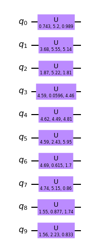
The resulting circuit has single-qubit gates only and is therefore depth 1.

x = np.frombuffer(x_solution_str, dtype=np.float32)
print('discretization:', x)
qc = QuantumCircuit.from_qasm_str(qasm_solution)
print('circuit:')
qc.draw(output='mpl')
discretization: [0.62056357 0.6314514  0.642224   ... 1.3485944  1.3865237  1.5813267 ]
circuit:

To verify correctnes I’ve collected several different methods of computing L2 norm here. In the code below I also only use qiskit methods for manipulating quantum ciruicts, so this should be a reliable check.

# This function assumes that all qubits are to be measured for the distribution.
def probabilities_from_circuit(qc):        
    state = Statevector.from_instruction(qc) 
    return state.probabilities()

def three_l2_errors_from_probabilities(p, x):
    error_2 = l2.idnm_l2_error(jnp.array(p), jnp.array(x))
    error_1 = l2.tnemoz_l2_error(p, x)
    error_0 = l2.l2_error(p, x)
    
    print(f'Error by method 0 (QuantumSage):{error_0}')
    print(f'Error by method 1 (tnemoz):{error_1}')
    print(f'Error by method 2 (idnm):{error_2}')
    
def three_l2_errors_from_circuit(qasm_str, x, reverse_bits=True):
    
    qc = QuantumCircuit.from_qasm_str(qasm_str)
    if reverse_bits:
        qc = qc.reverse_bits()
        
    print(f'Circuit depth is {qc.depth()}\n')
    p = probabilities_from_circuit(qc)
    three_l2_errors_from_probabilities(p, x)
    
three_l2_errors_from_circuit(qasm_solution, x)
Circuit depth is 1

Error by method 0 (QuantumSage):0.006361703002515892
Error by method 1 (tnemoz):0.005891621296138897
Error by method 2 (idnm):0.005880733951926231

Approach

I used fairly straightforward numerical optimization. I was interested if the target lognormal distribution can be approximated by small-depth circuits optimized directly. In other words, I minimized numerically the L2 error as a function of angles in the circuit and discretization intervals.

To my surprise, 9 and 10 qubits circuits with the smallest depth possible (containing only single-qubit gates) are able to give a good enough approximation below the threshold error. The freedom to adjust discretization seems crucial for low-depth circuits.

I also looked how well can one approximate the target distribution for a given number of qubits, assuming that the probability density can take any shape. This corresponds to the maximally expressive circuit, where all \(2^n\) amplitudes can be controlled precisely. Of course I didn’t optimize circuits of such depth. Rather, I optimized values of discrete functions directly. Interestingly, I found that the best possible approximation is not significanltly better than the approximation one can get with depth 1 circuits and the same number of qubits.

Setup

Lognormal distribution and L2 error

The following cells define the lognormal distribution \(f(x)\) itself as well as antiderivatives \(\int dx f(x)\) and \(\int dx f^2(x)\). Andtiderivatives will be useful for computing the L2 error.

def lognormal(x):
    s = 0.1
    mu = 0

    return 1 / (jnp.sqrt(2 * jnp.pi) * x * s) * jnp.exp(-(jnp.log(x) - mu) ** 2 / 2 / s ** 2)


def lognormal_int(x):
    return erf(5 * jnp.sqrt(2) * jnp.log(x)) / 2


def lognormal_squared_int(x):
    return erf(10 * jnp.log(x) + 1 / 20) / 2 / jnp.sqrt(jnp.pi) * 5 * jnp.power(jnp.e, 1 / 400)

# Uncomment to verify correctness of antiderivatives
# x = jnp.linspace(0.01, 2, 100)
# print(jnp.allclose(vmap(lognormal)(x), vmap(grad(lognormal_int))(x)))
# print(jnp.allclose(vmap(lognormal)(x)**2, vmap(grad(lognormal_squared_int))(x)))

Now we will define a simple class collecting some useful data about piecewise constant functions.

class DiscreteFunction:
    
    @staticmethod
    def condlist(x, grid):
        return [(g_left < x) & (x <= g_right) for g_left, g_right in zip(grid, grid[1:])]

    def __init__(self, grid, values):
        assert len(grid) == len(values) + 1, f'Number of grid points {len(grid)} does not match number of values {len(values)}.'
        self.grid = grid
        self.values = values
        self.probabilities = values * (grid[1:]-grid[:-1])
        
        def f(x):
            return jnp.piecewise(x, DiscreteFunction.condlist(x, grid), self.values)
        
        self.f = f
        
    def plot(self, x=None):
        if x is None:
            x = jnp.linspace(0.5, 1.5, 100)

        plt.plot(x, [self.f(xi) for xi in x]) # jit or vmap here gives an error for some reason. Without them unnecessarily slow.
        plt.plot(x, vmap(lognormal)(x))
            
    @classmethod            
    def from_probabilities(cls, grid, probs):
        values = probs/(grid[1:]-grid[:-1])
        return cls(grid, values)      

Here is the function that computes the L2 error between a given discrete function and the lognormal distribution. I used the equation

\[L2=\int_a^b (v-p(x))^2=D^{-1}p(x)^2\Big|^a_b-2 v D^{-1} p(x)\Big|^a_b+v^2 (b-a)\]

This is an error of approximating function \(p(x)\) by a constant \(v\) on an interval \((a,b)\). That this function is correct is confirmed by comparison with other independent methods which I presented above. This (a bit fancy) form is useful for speed in my numerical optimization.

def l2_error_contributions(discrete_function, left, right):
    
    grid = discrete_function.grid
    values = discrete_function.values
    
    # inner contributions
    f_squared_contrib = vmap(lognormal_squared_int)(grid[1:]) - vmap(lognormal_squared_int)(grid[:-1])
    f_contrib = vmap(lognormal_int)(grid[1:]) - vmap(lognormal_int)(grid[:-1])
    const_contrib = (values ** 2) * (grid[1:] - grid[:-1])

    # outer contributions
    outer_contrib_left = lognormal_squared_int(grid[0]) - lognormal_squared_int(left)
    outer_contrib_right = lognormal_squared_int(right) - lognormal_squared_int(grid[-1])

    # total
    total_contribs = f_squared_contrib - 2 * f_contrib * values + const_contrib + outer_contrib_left + outer_contrib_right

    return total_contribs


def l2_error(discrete_function, left=0, right=jnp.inf):
    return jnp.sqrt(l2_error_contributions(discrete_function, left, right).sum())

Here is a sample computation, x and p taken from here.

x = [0.1, 0.2, 0.3, 0.4, 0.5, 0.6, 0.7, 0.8, 0.9, 1. , 1.1, 1.2, 1.3, 1.4, 1.5, 1.6, 1.7]
p = [0., 0., 0., 0., 0., 0.081, 0.02, 0.1, 0.5, 0.115, 0.15, 0.03, 0.004, 0., 0., 0. ]
df = DiscreteFunction.from_probabilities(jnp.array(x), jnp.array(p))
df.plot()
print('L2 error:', l2_error(df))
L2 error: 0.93145823

Optimization setup (irrelevant)

I use JAX for numerical optimization. It is very flexible and efficient, by lacks some of the high level API present in other libraries. The code below is only to setup numerical minimization with JAX, it has no relation to the problem. It is included here only in order to make the notebook self-contained.

def update_step(loss_and_grad, opt, opt_state, params):
    loss, grads = loss_and_grad(params)
    updates, opt_state = opt.update(grads, opt_state)
    params = optax.apply_updates(params, updates)

    return params, loss, opt_state


def glue_params(params):
    return jnp.concatenate(params)


def unglue_params(glued_params, slice_indices):
    return [glued_params[i0:i1] for i0, i1 in zip(slice_indices, slice_indices[1:])]


def mynimize(loss, initial_params, opt_options):
    
    # Initialize optimizer and parameter splits.
    loss_and_grad = value_and_grad(loss)
    opt = opt_options.optimizer()
    opt_state = opt.init(initial_params)
    sizes = [len(ip) for ip in initial_params]
    slice_indices = [sum(sizes[:i]) for i in range(len(sizes)+1)]

    # Single learning iteration compatible with lax fori loop.
    def iteration_with_history(i, carry):
        glued_params_history, loss_history, opt_state = carry
        glued_params = glued_params_history[i]
        
        params = unglue_params(glued_params, slice_indices)
        
        params = initial_params._make(params)
        params, loss, opt_state = update_step(loss_and_grad, opt, opt_state, params)
        
        glued_params = glue_params(params)
        glued_params_history = glued_params_history.at[i+1].set(glued_params)
        
        loss_history = loss_history.at[i].set(loss)
        
        return glued_params_history, loss_history, opt_state

    # Initialize arrays holding whole histories for parameters and values.
    glued_initial_params = glue_params(initial_params)
    glued_params_history = jnp.zeros((opt_options.num_iterations, len(glued_initial_params))).at[0].set(glued_initial_params)
    loss_history = jnp.zeros((opt_options.num_iterations,))

    # Optimize iteratively within fori loop.
    glued_params_history, loss_history, _ = lax.fori_loop(
        0,
        opt_options.num_iterations,
        iteration_with_history,
        (glued_params_history, loss_history, opt_state))
    
    # Bring parameters to the original representation.
    params_history = vmap(lambda gp: unglue_params(gp, slice_indices))(glued_params_history)
    reordered_params_history = [initial_params._make([params_history[num_param][num_iteration] for num_param in range(len(initial_params))]) for num_iteration in range(opt_options.num_iterations)]

    return reordered_params_history, loss_history


@dataclass
class OptOptions:
    learning_rate: float = 0.01
    num_iterations: int = 2000
    random_seed: int = 0

    def optimizer(self):
        return optax.adam(self.learning_rate)
    
class OptResult:
    def __init__(self, raw_result, loss_func, opt_options):

        self.loss_func = loss_func
        self.opt_options = opt_options
        self.params_history = raw_result[0]
        self.loss_history = raw_result[1]
        
        self._best_i = jnp.argmin(self.loss_history)
        
        self.best_params = self.params_history[self._best_i]
        self.best_loss = self.loss_history[self._best_i]

    def _i_or_best_i(self, i):
        if i is None:
            return self._best_i
        else:
            return i

    def plot_loss_history(self):
        plt.plot(self.loss_history)
        plt.yscale('log')
        
    def __repr__(self):
        return f'OptResult: best_loss {self.best_loss}.'

Warm-up: fitting discrete functions directly

I found it very istructive to see what accuracy can be achieved if one can fully control values of the discrete function. Empirically, the best strtategy seems to

  • First optimize values of the discrete function with fixed discretization.
  • Continue by optimizing values and adjusting discretization intervals jointly.

Fitting values only

Here is the function that does the first part of the job.

V = namedtuple('Values', ['values'])

def fit_values(discrete_function, opt_options=OptOptions()):
    
    grid = discrete_function.grid
    initial_values = discrete_function.values
    
    @jit
    def loss(v):
        values = v.values
        df = DiscreteFunction(grid, values)
        return l2_error(df)
    
    initial_params = V(initial_values)
    results = mynimize(loss, initial_params, opt_options)
    return OptResult(results, loss, opt_options)

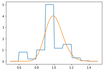
Here is the best this method can do with 10 qubits starting from random initial values between 0 and 1 (you can change the number of qubits if you wish). The histogram shows density of the grid points. At this point they are distributed uniformly.

num_qubits = 10

grid = jnp.linspace(0.5, 1.5, 2**num_qubits+1)
initial_values = random.uniform(random.PRNGKey(0), (2**num_qubits, ))
df = DiscreteFunction(grid, initial_values)
res = fit_values(df)
print(res)
df_fit = DiscreteFunction(df.grid, res.best_params.values)

res_values_only = res
df_fit_values_only = df_fit

plt.subplot(1, 2, 1)
res.plot_loss_history()
plt.title('loss history')
plt.subplot(1, 2, 2)
df_fit.plot()
plt.title('discretization')
plt.hist(np.array(df_fit.grid), bins=int(len(df_fit.grid)/5), density=True);
OptResult: best_loss 0.0033653806895017624.

Fitting values and grid

Now we introduce the second optimization procedure, which also adjusts discretization intervals.

One technical subtlety here is that the grid points should never go past each other. In order to prevent that I use auxilary variables, which are square roots of the distances between neighboring grid points, grid_roots. Even if some grid_root becomes negative the distance between the grid points grid_root**2 stays positive.

VG = namedtuple('ValuesGrid', ['values', 'grid_roots'])

def grid_to_roots(grid):
    all_points = jnp.concatenate([jnp.array([0]), grid]) # Append '0' to the left.
    cells = all_points[1:] - all_points[:-1]
    return jnp.sqrt(cells)

def roots_to_grid(roots):
    """ A bit of complicated syntaxis to restore grid from roots in a jax-compatible way."""
    cells = roots ** 2
    masks = jnp.tri(len(roots))
    pre_grid = vmap(lambda x: cells * x)(masks)
    return pre_grid.sum(axis=1)


def fit_values_and_grid(discrete_function, opt_options=OptOptions()):

    initial_grid_roots = grid_to_roots(discrete_function.grid)
    initial_values = discrete_function.values
    
    @jit
    def loss(vg):
        grid = roots_to_grid(vg.grid_roots)
        df = DiscreteFunction(grid, vg.values)
        return l2_error(df)
    
    initial_params = VG(initial_values, initial_grid_roots)
    results = mynimize(loss, initial_params, opt_options)
    return OptResult(results, loss, opt_options)

Here is the best fit to the lognormal distribution this procedure is able to find. Note that grid points are no longer distributed uniformly but clamp near the regions with the highest slope, as they should (this is in fact better visible at smaller qubit count). Note that here we initialized the optimization with values found at the previous stage. If we were to initialize them randomly, the result would be much worse. Note also a smaller learning rate at this stage.

num_qubits = 10

initial_grid = df_fit_values_only.grid
initial_values = df_fit_values_only.values

df = DiscreteFunction(initial_grid, initial_values)

opt_options = OptOptions(learning_rate=1e-4, num_iterations=5000)
res = fit_values_and_grid(df, opt_options)
print(res)

best_values = res.best_params.values
best_grid = roots_to_grid(res.best_params.grid_roots)
df_fit = DiscreteFunction(best_grid, best_values)

plt.subplot(1, 2, 1)
res.plot_loss_history()
plt.title('loss history')
plt.subplot(1, 2, 2)
df_fit.plot()
plt.title('discretization')
plt.hist(np.array(df_fit.grid), bins=int(len(df_fit.grid)/5), density=True);
OptResult: best_loss 0.00303847249597311.

Fitting quantum circuit

MyCircuit class

First I will define a very simple MyCircuit class that bundles qiskit representation with jax-compatible unitary. For the purposes of this notebook, we only need to place one gate on each qubit.

def U_gate(a):
    theta, phi, lmbda = a
    return jnp.array([[jnp.cos(theta/2), -jnp.exp(1j*lmbda)*jnp.sin(theta/2)],
                     [jnp.exp(1j*phi)*jnp.sin(theta/2), jnp.exp(1j*(phi+lmbda))*jnp.cos(theta/2)]])


class MyCircuit:
    def __init__(self, num_qubits):
        self.num_qubits = num_qubits
    
    def qiskit_circuit(self, angles):
        assert len(angles) == 3*self.num_qubits, f'Number of qubits {self.num_qubits} and angle triples {len(angles)} does not match.'
        qc = QuantumCircuit(self.num_qubits)
        angles = np.array(angles) # Qiskit does not accept JAX arrays.
        for i, (theta, phi, lmbda) in enumerate(angles.reshape(self.num_qubits, 3)):
            qc.u(theta, phi, lmbda, i)
        return qc
    
    def unitary(self, angles):
        gates = vmap(U_gate)(angles.reshape(self.num_qubits, 3))
        return reduce(jnp.kron, gates)
    
    def _verify(self, angles):
        u_qs = Operator(self.qiskit_circuit(angles).reverse_bits()).data
        u_jax = self.unitary(angles)
        return jnp.allclose(u_qs, u_jax)

Here is an example.

num_qubits = 5
angles = random.uniform(random.PRNGKey(0), (num_qubits*3, ), minval=0, maxval=2*jnp.pi)

mc = MyCircuit(num_qubits)
mc.unitary(angles)
print('qiskit unitary coincides with our unitary:', mc._verify(angles))
mc.qiskit_circuit(angles).draw(output='mpl')
qiskit unitary coincides with our unitary: True

Defining loss associated with a unitary

Quantum circuit transforms the input state. Amplitudes of the output state encode the values of the discrete function that we use to fit the lognormal distribution. Here we construct a function that takes a quantum circuit and returns the L2 error of the corresponding approximation.

def loss_from_unitary(grid, u):
    probs = probabilities_from_unitary(u)
    df = DiscreteFunction.from_probabilities(grid, probs)
    
    return l2_error(df)

def probabilities_from_unitary(u):
    all_zero_state = jnp.zeros(u.shape[0]).at[0].set(1)
    amplitudes = amplitudes_from_state(u @ all_zero_state)
    probabilities = jnp.abs(amplitudes)**2
    return probabilities

def amplitudes_from_state(state):
    return vmap(lambda basis_state: (state * basis_state).sum())(jnp.identity(len(state)))

Fitting angles only

Now we are ready to optimize angles in the circuit for the best fit to the target distribution. Discretization is held fixed at this stage.

A = namedtuple('Angles', ['angles'])

def fit_angles(grid, num_qubits, opt_options=OptOptions()):
    assert len(grid) == 2**num_qubits+1, f'Grid length {len(grid)} does not match number of qubits {num_qubits}.'
    circuit = MyCircuit(num_qubits)

    @jit
    def loss(a):
        u = circuit.unitary(a.angles)
        return loss_from_unitary(grid, u)

    initial_angles = random.uniform(random.PRNGKey(opt_options.random_seed), (3*num_qubits, ), minval=0, maxval=2*jnp.pi)
    initial_params = A(initial_angles)
    
    results = mynimize(loss, initial_params, opt_options)
    return OptResult(results, loss, opt_options)

Here is an example with 6 qubits.

num_qubits = 6
grid = jnp.linspace(0.6, 1.5, 2**num_qubits+1)
res = fit_angles(grid, num_qubits)

print(res)
circuit = MyCircuit(num_qubits)
probs = probabilities_from_unitary(circuit.unitary(res.best_params.angles))
df_fit = DiscreteFunction.from_probabilities(grid, probs)

plt.subplot(1, 2, 1)
res.plot_loss_history()
plt.title('loss history')
plt.subplot(1, 2, 2)
df_fit.plot()
plt.title('discretization')
plt.hist(np.array(df_fit.grid), bins=int(len(df_fit.grid)/5), density=True);

res_angles = res
df_fit_angles = df_fit
OptResult: best_loss 0.884075403213501.

The highly asymmetric shape of the fitting function here is typical and continutes to higher qubits. At the first glance, there seems to be little hope of making the construction work. However, as we see right now, adjusting the discretization ranges cuts the deal.

Fitting angles and grid

Here is the procedure that fits angles and grid together. We bundle it with the previous step into a single simple function fit_circuit that does all the work.

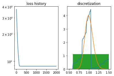
AG = namedtuple('AnglesGrid', ['angles', 'grid_roots'])

def fit_angles_and_grid(initial_angles, initial_grid, opt_options=OptOptions()):
    num_qubits = int(len(initial_angles)/3)
    assert len(initial_grid) == 2**num_qubits+1, f'Grid length {len(grid)} does not match number of qubits {num_qubits}.'
    circuit = MyCircuit(num_qubits)

    @jit
    def loss(ag):
        u = circuit.unitary(ag.angles)
        grid = roots_to_grid(ag.grid_roots)
        return loss_from_unitary(grid, u)
    
    initial_grid_roots = grid_to_roots(initial_grid)
    initial_params = AG(initial_angles, initial_grid_roots)
    
    results = mynimize(loss, initial_params, opt_options)
    return OptResult(results, loss, opt_options)

def fit_circuit(num_qubits):
    print('Initial optimization of angles:')
    grid = jnp.linspace(0.6, 1.5, 2**num_qubits+1)
    res = fit_angles(grid, num_qubits)
    print(res)
    
    print('\nOptimization of angles and grid:')
    circuit = MyCircuit(num_qubits)

    initial_angles = res.best_params.angles
    initial_grid = grid

    opt_options = OptOptions(learning_rate=1e-4, num_iterations=10000)
    
    res = fit_angles_and_grid(initial_angles, initial_grid, opt_options)

    print(res)

    best_probs = probabilities_from_unitary(circuit.unitary(res.best_params.angles))
    best_grid = roots_to_grid(res.best_params.grid_roots)

    df_fit = DiscreteFunction.from_probabilities(best_grid, best_probs)

    plt.subplot(1, 2, 1)
    res.plot_loss_history()
    plt.title('loss history')
    plt.subplot(1, 2, 2)
    df_fit.plot()
    plt.hist(np.array(df_fit.grid), bins=int(len(df_fit.grid)/5), density=True);
    plt.title('discretization')
    
    return circuit.qiskit_circuit(res.best_params.angles).qasm(), best_grid

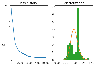
Here is what happens for 6 qubits when we follow up initial angle optimization with the grid optimization.

qasm, grid = fit_circuit(6)
Initial optimization of angles:
OptResult: best_loss 0.884075403213501.

Optimization of angles and grid:
OptResult: best_loss 0.04849757254123688.

The optimization results improved dramatically. We are able to achive \(5\times 10^{-2}\) error already on six qubits. As we can anticipate, using all 10 qubits helps a lot.
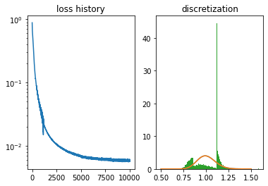
Final solution

Here is the final solution. The qasm file and grid specified at the beginning of this notebook were produced here. On Colab’s GPU this takes about 10 minutes to run.

qasm, grid = fit_circuit(10)
Initial optimization of angles:
OptResult: best_loss 0.8839455246925354.

Optimization of angles and grid:
OptResult: best_loss 0.005602838937193155.

print('grid:\n')
print(np.array(grid).tobytes())
print('\nQASM: \n')
qasm
grid:

b'A\xdd\x1e?\xcd\xa6!?\xcbh$?\xc4 \'?\x11\xcd)?\xe7j,?n\xf2.?\xeeY1?\xcd\x963?t\xb35?\xc8\x847?Z\x029?\xf0/:?\x9f!;?!\xe6;?\x96\x8d<?\xd3 =?\xbd\xd5=?\xdet>?\x1c\x03??\x8a\x83??.\xfc??\xa2j@?\x89\xd0@?\xeb.A?\xd7\x97A?\x03\xf9A?\x87SB?\x0f\xa8B?\xc2\xf9B?sFC?\xc0\x8eC?\xfb\xd2C?k\x15D?UTD?\x1c\x90D?\xed\xc8D?\xb8\x00E?\xdf5E?\xa6hE?%\x99E?\xca\xd0E?\xd4\x05F?\x898F?\xffhF?\xd4\x98F?\x9f\xc6F?\x8d\xf2F?\xb3\x1cG?\xb4TG?!\x8aG?>\xbdG?!\xeeG?k\x1eH?\xadLH?\x16yH?\xb7\xa3H?\xde\xd4H?\xf5\x03I?,1I?\x92\\I?\x94\x87I?\xe6\xb0I?\xb2\xd8I?\xfd\xfeI?+ J?1@J?*_J?\x16}J?\xee\x9aJ?\xc8\xb7J?\xb9\xd3J?\xc3\xeeJ?6\x0eK?\x99,K?\x03JK?xfK?\xde\x82K?Z\x9eK?\xfe\xb8K?\xcb\xd2K?q\xf5K?\xe4\x16L?>7L?\x80VL?\xafuL?\xd4\x93L?\x07\xb1L?J\xcdL?)\xeeL?\xec\rM?\xae,M?lJM?\x1fhM?\xdc\x84M?\xba\xa0M?\xb5\xbbM?\xa4\xd6M?\xbc\xf0M?\x0f\nN?\x9d"N?0;N?\x05SN?,jN?\xa5\x80N?\xdd\x9aN?G\xb4N?\xf5\xccN?\xe6\xe4N?\xdd\xfcN?\x1e\x14O?\xb9*O?\xab@O?:^O?\xd9zO?\x9e\x96O?\x86\xb1O?q\xccO?\x89\xe6O?\xe0\xffO?v\x18P?"5P?\xe9PP?\xe1kP?\x07\x86P?1\xa0P?\x93\xb9P?<\xd2P?*\xeaP?\xd6\x01Q?\xd1\x18Q?*/Q?\xe0DQ?\xa4ZQ?\xc9oQ?_\x84Q?a\x98Q?\xc4\xafQ?{\xc6Q?\x93\xdcQ?\n\xf2Q?\x91\x07R?~\x1cR?\xdc0R?\xaaDR?b_R?MyR?\x80\x92R?\xf4\xaaR?x\xc3R?C\xdbR?i\xf2R?\xe5\x08S?+#S?\xab<S?tUS?\x87mS?\xa8\x85S?\x17\x9dS?\xe6\xb3S?\x0f\xcaS?@\xe0S?\xd2\xf5S?\xd3\nT?@\x1fT?\xc03T?\xaeGT?\x1d[T?\x03nT?"\x84T?\xa1\x99T?\x91\xaeT?\xef\xc2T?`\xd7T?B\xebT?\xa4\xfeT?~\x11U?\xf5*U?\xb2CU?\xc4[U?(sU?\x9d\x8aU?l\xa1U?\x9f\xb7U?7\xcdU?v\xe6U?\xfe\xfeU?\xdd\x16V?\x12.V?ZEV?\xfc[V?\x06rV?w\x87V?8\x9aV?{\xacV?K\xbeV?\xa3\xcfV?\x11\xe1V?\r\xf2V?\x9f\x02W?\xc3\x12W?\xad%W?\x188W?\rJW?\x8c[W?!mW?B~W?\xf9\x8eW?B\x9fW?I\xb5W?\xb6\xcaW?\x98\xdfW?\xec\xf3W?T\x08X?4\x1cX?\x94/X?qBX?\x89XX?\tnX?\xfc\x82X?`\x97X?\xdd\xabX?\xcd\xbfX?@\xd3X?0\xe6X?1\xf9X?\xb3\x0bY?\xc1\x1dY?X/Y?\tAY?CRY?\x16cY?ysY?\xb0\x86Y?g\x99Y?\xaa\xabY?t\xbdY?U\xcfY?\xc4\xe0Y?\xc7\xf1Y?[\x02Z?\xc9\x18Z?\x9f.Z?\xe7CZ?\xa1XZ?smZ?\xba\x81Z?\x81\x95Z?\xc3\xa8Z?S\xbfZ?K\xd5Z?\xb6\xeaZ?\x90\xffZ?\x85\x14[?\xeb([?\xd4<[?7P[?\xe0\x99[?\xae\xe0[?\xe6$\\?\x95f\\?\xe2\xa7\\?\xd1\xe6\\?\x9b#]?E^]?W\xa2]?\xef\xe3]?J#^?p`^?Z\x9d^?1\xd8^?#\x11_?1H_?\x05\x92_?)\xd9_?\xdf\x1d`?.``?=\xa2`?\n\xe2`?\xcb\x1fa?\x80[a?\xec\xa0a?\xf4\xe3a?\xd5$b?\x8fcb?*\xa2b?\xbd\xdeb?v\x19c?VRc?\x1a\x8bc?\x1a\xc2c?\x82\xf7c?L+d?$_d?o\x91d?S\xc2d?\xca\xf1d?4)e?\xf4^e?/\x93e?\xdf\xc5e?\xac\xf8e?\xfd)f?\xf7Yf?\x96\x88f?p\xc7f?`\x04g?\x90?g?\x00yg?\x86\xb2g?\\\xeag?\xaa h?hUh?\x08\x93h?\xd4\xceh?\xfa\x08i?rAi?\x12zi?\x12\xb1i?\x9c\xe6i?\xa8\x1aj?.Hj?|tj?\xb0\x9fj?\xc4\xc9j?\n\xf4j?6\x1dk?`Ek?\x86lk?`\x9ak?\n\xc7k?\x9a\xf2k?\x08\x1dl?\xb2Gl?Bql?\xd2\x99l?\\\xc1l?\xdc\xf6l?\xed*m?\xb4]m?%\x8fm?\xd6\xc0m?@\xf1m?z n?~Nn?o\x84n?\xf7\xb8n?6\xecn?%\x1eo?ZPo?I\x81o?\x0f\xb1o?\xa1\xdfo?h\x0ep?\x06<p?\x95hp?\x0b\x94p?\xc9\xbfp?x\xeap?,\x14q?\xdf<q?\xa2lq?<\x9bq?\xc4\xc8q?/\xf5q?\xec!r?\x94Mr?Axr?\xe9\xa1r?`\xdar?t\x11s?CGs?\xc3{s?\xa0\xb0s?7\xe4s?\xa5\x16t?\xdfGt?\xac\x81t?\x15\xbat?7\xf1t?\x0b\'u?F]u?7\x92u?\x01\xc6u?\x93\xf8u?\xe7*v?\x10\\v?,\x8cv?*\xbbv?\x8f\xeav?\xdc\x18w?0Fw?\x7frw?\x97\xa6w?|\xd9w?S\x0bx?\x04<x?&mx?-\x9dx?5\xccx?0\xfax?\xa38y?\xafuy?t\xb1y?\xe4\xeby?\xdd&z?\x87`z?\x02\x99z?B\xd0z?F\x11{?\xdcP{?,\x8f{?!\xcc{?\xb0\t|?\xebE|?\xf6\x80|?\xc0\xba|?\x08\xf5|?\x15.}?\x06f}?\xcb\x9c}?\x1e\xd4}?M\n~?r?~?\x80s~?\xd2\xb0~?\xe2\xec~?\xd4\'\x7f?\x90a\x7f?\xf2\x9b\x7f?#\xd5\x7f?\xa3\x06\x80?$"\x80?\x98G\x80?Pl\x80?]\x90\x80?\xb9\xb3\x80?\x81\xd7\x80?\x9d\xfa\x80?\x18\x1d\x81?\xeb>\x81?\xdbf\x81?\x0b\x8e\x81?\x91\xb4\x81?f\xda\x81?\xb7\x00\x82?]&\x82?`K\x82?\xb6o\x82?\xd0\x8f\x82?S\xaf\x82?K\xce\x82?\xb6\xec\x82?\x8d\x0b\x83?\xd7)\x83?\xa1G\x83?\xddd\x83?q\x87\x83?m\xa9\x83?\xdc\xca\x83?\xbe\xeb\x83?\x19\r\x84?\xde-\x84?"N\x84?\xd7m\x84?5\x99\x84?\xed\xc3\x84?\t\xee\x84?\x84\x17\x85?\xaaA\x85?4k\x85?.\x94\x85?\x8f\xbc\x85?t\xec\x85?\xb6\x1b\x86?fJ\x86?|x\x86?f\xa7\x86?\xb8\xd5\x86?\x87\x03\x87?\xbe0\x87?\xc1^\x87?/\x8c\x87?\x1f\xb9\x87?\x88\xe5\x87?\xca\x12\x88?\x87?\x88?\xc6k\x88?\x88\x97\x88?\x95\xcb\x88?"\xff\x88?B2\x89?\xe6d\x89?\xa8\x98\x89?\xf8\xcb\x89?\xe0\xfe\x89?W1\x8a?\x02w\x8a?g\xbc\x8a?\xac\x01\x8b?\xb8F\x8b?\xcd\x8d\x8b?\xb9\xd4\x8b?\xa6\x1b\x8c?{b\x8c?\xcf\xb7\x8c?p\r\x8d?\x91c\x8d?#\xba\x8d?\x06\x14\x8e?\x8en\x8e?\xf5\xc9\x8e?+&\x8f?{&\x8f?\xca&\x8f?\x18\'\x8f?d\'\x8f?\xb1\'\x8f?\xfc\'\x8f?G(\x8f?\x8e(\x8f?\xe3(\x8f?6)\x8f?\x87)\x8f?\xd9)\x8f?)*\x8f?x*\x8f?\xc6*\x8f?\x11+\x8f?x+\x8f?\xdd+\x8f?A,\x8f?\xa3,\x8f?\x04-\x8f?d-\x8f?\xc4-\x8f? .\x8f?\x8d.\x8f?\xf8.\x8f?`/\x8f?\xc6/\x8f?00\x8f?\x940\x8f?\xf70\x8f?Y1\x8f?\xbb1\x8f?\x1a2\x8f?y2\x8f?\xd62\x8f?43\x8f?\x8e3\x8f?\xe83\x8f??4\x8f?\xa64\x8f?\x0b5\x8f?n5\x8f?\xcf5\x8f?36\x8f?\x936\x8f?\xf16\x8f?N7\x8f?\xcb7\x8f?F8\x8f?\xbe8\x8f?49\x8f?\xac9\x8f?":\x8f?\x94:\x8f?\x05;\x8f?\x89;\x8f?\t<\x8f?\x89<\x8f?\x07=\x8f?\x82=\x8f?\xfe=\x8f?x>\x8f?\xee>\x8f?V?\x8f?\xbb?\x8f? @\x8f?\x83@\x8f?\xe4@\x8f?EA\x8f?\xa5A\x8f?\x01B\x8f?qB\x8f?\xdcB\x8f?EC\x8f?\xabC\x8f?\x14D\x8f?yD\x8f?\xdfD\x8f??E\x8f?\xc3E\x8f?FF\x8f?\xc6F\x8f?DG\x8f?\xc2G\x8f?=H\x8f?\xb8H\x8f?-I\x8f?\xbbI\x8f?DJ\x8f?\xcbJ\x8f?NK\x8f?\xd4K\x8f?XL\x8f?\xd5L\x8f?TM\x8f?\xd3M\x8f?NN\x8f?\xc8N\x8f??O\x8f?\xb7O\x8f?-P\x8f?\xa0P\x8f?\x13Q\x8f?\x97Q\x8f?\x19R\x8f?\x9aR\x8f?\x17S\x8f?\x95S\x8f?\x11T\x8f?\x8bT\x8f?\x01U\x8f?\xa3U\x8f?AV\x8f?\xdeV\x8f?xW\x8f?\x11X\x8f?\xa8X\x8f?<Y\x8f?\xccY\x8f?xZ\x8f?\x1e[\x8f?\xc3[\x8f?b\\\x8f?\x06]\x8f?\xa4]\x8f??^\x8f?\xd9^\x8f?r_\x8f?\x07`\x8f?\x99`\x8f?\'a\x8f?\xb9a\x8f?Gb\x8f?\xd2b\x8f?Yc\x8f?\xfbc\x8f?\x97d\x8f?1e\x8f?\xc7e\x8f?`f\x8f?\xf5f\x8f?\x88g\x8f?\x17h\x8f?\xd9h\x8f?\x99i\x8f?Uj\x8f?\x0bk\x8f?\xc5k\x8f?zl\x8f?-m\x8f?\xdbm\x8f?\xaan\x8f?ro\x8f?8p\x8f?\xfap\x8f?\xbcq\x8f?|r\x8f?8s\x8f?\xf0s\x8f?\xa9t\x8f?^u\x8f?\x11v\x8f?\xc0v\x8f?pw\x8f?\x1cx\x8f?\xc6x\x8f?ky\x8f?0z\x8f?\xefz\x8f?\xaa{\x8f?b|\x8f?\x1d}\x8f?\xd2}\x8f?\x85~\x8f?4\x7f\x8f?!\x80\x8f?\n\x81\x8f?\xee\x81\x8f?\xce\x82\x8f?\xb0\x83\x8f?\x8d\x84\x8f?f\x85\x8f?<\x86\x8f?5\x87\x8f?-\x88\x8f?\x1d\x89\x8f?\t\x8a\x8f?\xf6\x8a\x8f?\xe1\x8b\x8f?\xc4\x8c\x8f?\xa6\x8d\x8f?l\x8e\x8f?.\x8f\x8f?\xeb\x8f\x8f?\xa4\x90\x8f?a\x91\x8f?\x19\x92\x8f?\xcc\x92\x8f?~\x93\x8f?M\x94\x8f?\x19\x95\x8f?\xe0\x95\x8f?\xa4\x96\x8f?k\x97\x8f?.\x98\x8f?\xea\x98\x8f?\xa6\x99\x8f?\xa2\x9a\x8f?\x99\x9b\x8f?\x8d\x9c\x8f?{\x9d\x8f?l\x9e\x8f?Y\x9f\x8f??\xa0\x8f?!\xa1\x8f?.\xa2\x8f?2\xa3\x8f?3\xa4\x8f?-\xa5\x8f?,\xa6\x8f?#\xa7\x8f?\x18\xa8\x8f?\x06\xa9\x8f?\xf8\xa9\x8f?\xe4\xaa\x8f?\xcc\xab\x8f?\xae\xac\x8f?\x94\xad\x8f?s\xae\x8f?Q\xaf\x8f?)\xb0\x8f?\'\xb1\x8f? \xb2\x8f?\x14\xb3\x8f?\x03\xb4\x8f?\xf5\xb4\x8f?\xe2\xb5\x8f?\xca\xb6\x8f?\xad\xb7\x8f?\xe2\xb8\x8f?\x13\xba\x8f?<\xbb\x8f?^\xbc\x8f?\x85\xbd\x8f?\xa6\xbe\x8f?\xc1\xbf\x8f?\xd6\xc0\x8f?\x1d\xc2\x8f?\\\xc3\x8f?\x97\xc4\x8f?\xc8\xc5\x8f?\x01\xc7\x8f?0\xc8\x8f?Y\xc9\x8f?}\xca\x8f?\xe4\xce\x8f?2\xd3\x8f?n\xd7\x8f?\x95\xdb\x8f?\xc7\xdf\x8f?\xe5\xe3\x8f?\xf1\xe7\x8f?\xe6\xeb\x8f?\x92\xf0\x8f?&\xf5\x8f?\xaa\xf9\x8f?\x15\xfe\x8f?\x8d\x02\x90?\xf0\x06\x90?<\x0b\x90?u\x0f\x90?4\x15\x90?\xd8\x1a\x90?b \x90?\xd1%\x90?S+\x90?\xb80\x90?\x086\x90?8;\x90?^A\x90?dG\x90?PM\x90? S\x90?\x00Y\x90?\xc6^\x90?qd\x90?\x01j\x90?\x9fo\x90?"u\x90?\x8dz\x90?\xdd\x7f\x90?@\x85\x90?\x87\x8a\x90?\xb7\x8f\x90?\xcc\x94\x90?\xcd\x9a\x90?\xb1\xa0\x90?{\xa6\x90?)\xac\x90?\xe6\xb1\x90?\x8c\xb7\x90?\x15\xbd\x90?\x86\xc2\x90?\xee\xc9\x90?4\xd1\x90?]\xd8\x90?c\xdf\x90?\x80\xe6\x90?y\xed\x90?X\xf4\x90?\x13\xfb\x90?\x08\x03\x91?\xd8\n\x91?\x88\x12\x91?\x10\x1a\x91?\xb5!\x91?6)\x91?\x960\x91?\xd67\x91?6>\x91?\x7fD\x91?\xa9J\x91?\xb3P\x91?\xd5V\x91?\xd6\\\x91?\xbeb\x91?\x8bh\x91?bo\x91?\x1av\x91?\xb3|\x91?.\x83\x91?\xbf\x89\x91?2\x90\x91?\x84\x96\x91?\xbc\x9c\x91?5\xa5\x91?\x88\xad\x91?\xb9\xb5\x91?\xc2\xbd\x91?\xe8\xc5\x91?\xeb\xcd\x91?\xc8\xd5\x91?\x82\xdd\x91?\xa5\xe6\x91?\x9f\xef\x91?r\xf8\x91? \x01\x92?\xea\t\x92?\x8f\x12\x92?\n\x1b\x92?e#\x92?\xd5+\x92?!4\x92?H<\x92?MD\x92?nL\x92?fT\x92?>\\\x92?\xf4c\x92?\x0em\x92?\x01v\x92?\xcf~\x92?u\x87\x92?8\x90\x92?\xd5\x98\x92?P\xa1\x92?\xa0\xa9\x92?\xfd\xb4\x92?-\xc0\x92?0\xcb\x92?\x00\xd6\x92?\xfe\xe0\x92?\xc9\xeb\x92?i\xf6\x92?\xdf\x00\x93?@\r\x93?i\x19\x93?g%\x93?41\x93?-=\x93?\xf4H\x93?\x8fT\x93?\xfa_\x93?kk\x93?\xacv\x93?\xc2\x81\x93?\xa9\x8c\x93?\xb7\x97\x93?\x98\xa2\x93?O\xad\x93?\xd7\xb7\x93?M\xc4\x93?\x92\xd0\x93?\xa9\xdc\x93?\x90\xe8\x93?\xa3\xf4\x93?\x86\x00\x94?>\x0c\x94?\xc2\x17\x94?\x83\'\x94?\x087\x94?ZF\x94?rU\x94?\xcfd\x94?\xefs\x94?\xda\x82\x94?\x8f\x91\x94?\xfe\xa2\x94?2\xb4\x94?+\xc5\x94?\xee\xd5\x94?\xf7\xe6\x94?\xc6\xf7\x94?`\x08\x95?\xbd\x18\x95?^)\x95?\xc29\x95?\xf2I\x95?\xe7Y\x95?%j\x95?%z\x95?\xf5\x89\x95?\x88\x99\x95?\x06\xac\x95?D\xbe\x95?M\xd0\x95?\x19\xe2\x95?9\xf4\x95?\x1c\x06\x96?\xc9\x17\x96?9)\x96?*A\x96?\xdbX\x96?Tp\x96?\x8f\x87\x96?E\x9f\x96?\xbc\xb6\x96?\xfb\xcd\x96?\xfd\xe4\x96?e\x00\x97?\x93\x1b\x97?\x896\x97?GQ\x97?\xa2l\x97?\xc2\x87\x97?\xad\xa2\x97?_\xbd\x97?"\xd5\x97?\xaa\xec\x97?\x02\x04\x98?\x18\x1b\x98?\xae2\x98?\x08J\x98?.a\x98?\x19x\x98?j\x93\x98?\x80\xae\x98?n\xc9\x98?\x1b\xe4\x98?o\xff\x98?\x89\x1a\x99?v5\x99?-P\x99?\x10u\x99?\xd9\x99\x99?\x93\xbe\x99?.\xe3\x99?\xdc\x08\x9a?p.\x9a?\xfbS\x9a?qy\x9a?{\xa6\x9a?\x9d\xd3\x9a?\xe2\x00\x9b?=.\x9b?)]\x9b?9\x8c\x9b?\x81\xbb\x9b?\xf5\xea\x9b?\r\x1c\x9c?ZM\x9c?\xfd~\x9c?\xe0\xb0\x9c?\xac\xe4\x9c?\xca\x18\x9d?[M\x9d?O\x82\x9d?\xb7\xc2\x9d?\x03\x04\x9e?hF\x9e?\xd8\x89\x9e?\xa8\xd0\x9e?\xd5\x18\x9f?\x8ab\x9f?\xce\xad\x9f?\xa2\x19\xa0?\x16\x8a\xa0?\xf0\xff\xa0?\xc9{\xa1?\xd8\x02\xa2?\x87\x92\xa2?\xa4,\xa3?\r\xd3\xa3?\xcb\xaf\xa4?Y\xaa\xa5?`\xce\xa6?\xc1.\xa8?8\x01\xaa?\xbe\x9e\xac?\x9cy\xb1?\xeah\xca?'

QASM: 
'OPENQASM 2.0;\ninclude "qelib1.inc";\nqreg q[10];\nu(0.74283063,5.2044897,0.98926634) q[0];\nu(3.6797547,5.5519018,5.144691) q[1];\nu(1.8728536,5.2152901,1.8132132) q[2];\nu(4.5905914,0.059626058,4.4641838) q[3];\nu(4.6174035,4.488265,4.80723) q[4];\nu(4.5903974,2.4311147,5.9549437) q[5];\nu(4.687211,0.61535245,1.6999713) q[6];\nu(4.7381563,5.1480927,0.86016178) q[7];\nu(1.550415,0.87675416,1.7371591) q[8];\nu(1.5602221,2.2341533,0.83279055) q[9];\n'
No matching items